
What's the Area? (Part VI)
This is Part 6 of a series on calculating area and integration. In the first part, I introduced the problem. In the second part, I used geometry to calculate the area of a trapezoid. In Part 3, we looked to calculus for a solution. In Part 4, we employed a shotgun approach and randomly sampled the space for Monte Carlo integration. In Part 5, we tried uniform sampling (the peg board approach) and found it didn't work as well as random sampling.
An impetus behind writing this series involves the relationship between theory and practice and how the two are typically taught. Theory often seems to run East and West while practice runs North and South. When one learns geometry, one learns all of the ins and outs of geometry. So it goes with calculus, statistics, numerical methods, etc.
In education and inquiry, topics are typically addressed along the "theory axis," and issues are rarely addressed along the "practice axis" due to the dynamics of specialization. Your best bet for a course discussing along the practice axis might be a course in applied mathematics or numerical methods or mathematics for engineers. For me this series of posts is an initial experiment in looking at a simple problem and trying to examine it along the axis of practice with a comparative approach.
After trying the shotgun approach and the peg board approach to Monte Carlo, I closed asking if there's a better way to sample the space. The answer comes in a technique called Quasi-Monte Carlo Integration.
In the sampling of space in Monte Carlo Integration (what I called the shotgun approach), random points were selected using pseudo-random numbers. If you don't know what pseudo-random numbers are, it will have to suffice to say these are fake random numbers generated by computers that are for most practical purposes just as good as the real thing. Computers, being deterministic, can't generate random numbers in the traditional sense of the word. (What random means exactly is a whole other philosophical abyss that will be quite intentionally avoided here.)
While Monte Carlo Integration uses pseudo-random numbers to generate sample points, Quasi-Monte Carlo uses quasi-random numbers. One thing about quasi-random numbers is that they're among the most poorly named mathematical entities, so perhaps you should erase the term quasi-random from memory now and learn to call them low discrepancy sequences from the beginning (although the Wikipedia entry is tagged as being in need of expert attention, it still has interesting information in it).
One of the simplest quasi-random / low discrepancy sequences is the Halton sequence, named after John H. Halton. I've chosen the Halton sequence as an example because it is simply explained, my intention is only to demonstrate a general principle, and I don't think I'll have time to do anything more than list the names of other low discrepancy sequences (cf. Hammersley, Sobol, Faure, Neiderreiter).
To generate the Halton sequence, convert a number from base 10 to a prime number base, mirror the number about the decimal point, and finally convert the number back to base 10.
An example is illuminating. Let's use base 2, because it's familiar to computer geeks and bits are computationally attractive.
1 -> 001.0 -> 0.100 -> 0.500
2 -> 010.0 -> 0.010 -> 0.250
3 -> 011.0 -> 0.110 -> 0.750
4 -> 100.0 -> 0.010 -> 0.125
5 -> 101.0 -> 0.101 -> 0.625
6 -> 110.0 -> 0.011 -> 0.375
7 -> 111.0 -> 0.111 -> 0.875
If you examine the sequence for a while, you'll see why quasi-random is a poor name. In the case of base 2, the first point is in the middle, the next is half way between the middle and the lower bound, the next is half way between the middle and the upper bound, etc. Similar results are found with other bases.
It's quite beautiful in terms of simplicity and results. If you think about the problems we encountered with the peg board approach of uniform sampling, you should see the value in using low discrepancy sequences for sampling.
Quasi-random sequences tend to converge more quickly than uniform sampling (the peg board approach) and pseudo-random sequences (the shotgun approach), and they're more orderly than pseudo-random sequences (which is why low discrepancy is a better term than quasi-random).
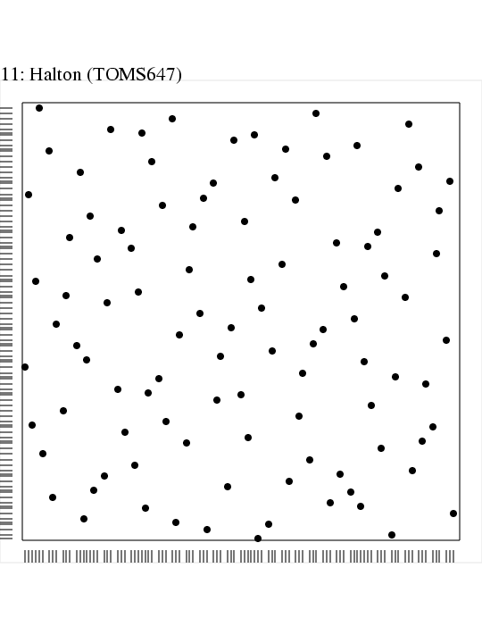
Here's a nice page at FSU with links to 2D plots of sample points resulting from quasi-random sequences in the unit square. (Also: Here's a little applet I cranked out [i.e., may contain bugs, but seems to match Burkardt's page] that demonstrates 2D points using the Halton sequence [base 2 for x and base 3 for y].)
At this point, I feel I'm beginning to deviate from the subject of calculating area and integration into the subject of point samping. Oh well, this is useful stuff to know and applicable in many areas from computer graphics to stochastic geometry to statistical mechanics to financial engineering.
An impetus behind writing this series involves the relationship between theory and practice and how the two are typically taught. Theory often seems to run East and West while practice runs North and South. When one learns geometry, one learns all of the ins and outs of geometry. So it goes with calculus, statistics, numerical methods, etc.
In education and inquiry, topics are typically addressed along the "theory axis," and issues are rarely addressed along the "practice axis" due to the dynamics of specialization. Your best bet for a course discussing along the practice axis might be a course in applied mathematics or numerical methods or mathematics for engineers. For me this series of posts is an initial experiment in looking at a simple problem and trying to examine it along the axis of practice with a comparative approach.
After trying the shotgun approach and the peg board approach to Monte Carlo, I closed asking if there's a better way to sample the space. The answer comes in a technique called Quasi-Monte Carlo Integration.
In the sampling of space in Monte Carlo Integration (what I called the shotgun approach), random points were selected using pseudo-random numbers. If you don't know what pseudo-random numbers are, it will have to suffice to say these are fake random numbers generated by computers that are for most practical purposes just as good as the real thing. Computers, being deterministic, can't generate random numbers in the traditional sense of the word. (What random means exactly is a whole other philosophical abyss that will be quite intentionally avoided here.)
While Monte Carlo Integration uses pseudo-random numbers to generate sample points, Quasi-Monte Carlo uses quasi-random numbers. One thing about quasi-random numbers is that they're among the most poorly named mathematical entities, so perhaps you should erase the term quasi-random from memory now and learn to call them low discrepancy sequences from the beginning (although the Wikipedia entry is tagged as being in need of expert attention, it still has interesting information in it).
One of the simplest quasi-random / low discrepancy sequences is the Halton sequence, named after John H. Halton. I've chosen the Halton sequence as an example because it is simply explained, my intention is only to demonstrate a general principle, and I don't think I'll have time to do anything more than list the names of other low discrepancy sequences (cf. Hammersley, Sobol, Faure, Neiderreiter).
To generate the Halton sequence, convert a number from base 10 to a prime number base, mirror the number about the decimal point, and finally convert the number back to base 10.
An example is illuminating. Let's use base 2, because it's familiar to computer geeks and bits are computationally attractive.
1 -> 001.0 -> 0.100 -> 0.500
2 -> 010.0 -> 0.010 -> 0.250
3 -> 011.0 -> 0.110 -> 0.750
4 -> 100.0 -> 0.010 -> 0.125
5 -> 101.0 -> 0.101 -> 0.625
6 -> 110.0 -> 0.011 -> 0.375
7 -> 111.0 -> 0.111 -> 0.875
If you examine the sequence for a while, you'll see why quasi-random is a poor name. In the case of base 2, the first point is in the middle, the next is half way between the middle and the lower bound, the next is half way between the middle and the upper bound, etc. Similar results are found with other bases.
It's quite beautiful in terms of simplicity and results. If you think about the problems we encountered with the peg board approach of uniform sampling, you should see the value in using low discrepancy sequences for sampling.
Quasi-random sequences tend to converge more quickly than uniform sampling (the peg board approach) and pseudo-random sequences (the shotgun approach), and they're more orderly than pseudo-random sequences (which is why low discrepancy is a better term than quasi-random).
Here's a nice page at FSU with links to 2D plots of sample points resulting from quasi-random sequences in the unit square. (Also: Here's a little applet I cranked out [i.e., may contain bugs, but seems to match Burkardt's page] that demonstrates 2D points using the Halton sequence [base 2 for x and base 3 for y].)
At this point, I feel I'm beginning to deviate from the subject of calculating area and integration into the subject of point samping. Oh well, this is useful stuff to know and applicable in many areas from computer graphics to stochastic geometry to statistical mechanics to financial engineering.
posted by metamerist at
1:27 PM
![]()

0 Comments:
Post a Comment
Subscribe to Post Comments [Atom]
<< Home